speccon

Contents

What is speccon?

‘speccon’ is the common name for a number of programs that use the spectral Galerkin method to solve multilayer consolidation problems.

Speccon programs currently available in geotecha are:

• speccon1d_vr - Multilayer consolidation with vertical drains.

• See geotecha.speccon.speccon1d_vr.Speccon1dVR for details and input variables.

• speccon1d_vrw - Multilayer consolidation with vertical drains including well resistance.

• See geotecha.speccon.speccon1d_vrw.Speccon1dVRW for details and input variables.

• speccon1d_vrc - Multilayer consolidation with stone columns including vertical and radial drainage in the column.

• See geotecha.speccon.speccon1d_vrc.Speccon1dVRC for details and input variables.

• speccon1d_unsat - Multilayer consolidation of unsaturated soil.

• See geotecha.speccon.speccon1d_unsat.Speccon1dUnsat for details and input variables.

How to use speccon programs?

There are two main ways to use speccon programs:

• Use a speccon.exe script

• Create an input file containing python syntax initializing relevant variables. Only a subset of python syntax is allowed.
• Run the relevant speccon.exe script with the input file.
• Output such as csv data files, parsed input files, and plots are controlled by various input variables.
• This is the best option for working with one set of input at a time.
• The speccon.exe scripts should have been installed with geotecha. They can usually be found in the /python27/Scripts/ or similar folder. Alternately run them directly from a command prompt (assuming their location is in your path environment variable).

• Use the Speccon classes in your own python programs/scripts.

• Instead of passing an input file to a script you can initialize a speccon object with a multi-line string.
• Create a multi-line string containing python syntax to initialize relevant variables. Remember that the string itself cannot contain all python syntax. This is not as restrictive as it first appears as you can easily pass calculated values into the string using the format method essentially giving you access to all python functionality.
• After initializing a speccon object perform the analysis with the make_all method. a subset of teh python language
• This is the most flexible approach especially for parametric studies and custom plots.

The relevant variables for use in each speccon program can be found in the docstring of the relevant file which can be found in the api section of the docs.

Examples

Specific Examples can be found in the Geotecha Examples section. Further examples can be found by digging around in the testing routines in the source code.

Using speccon1d_vr below are three different ways to run a speccon analysis.

Script

Create a text file containing the text below. Locate and run the speccon1d_vr.exe file. Choose the just created input file. A folder of output should be created in the same directory as the input file.

# Example input file for speccon1d_vr.  Use speccon1d_vr.exe to run.

# Vertical consolidation of four soil layers
# Figure 2 from:
# Schiffman, R. L, and J. R Stein. (1970) 'One-Dimensional Consolidation of
# Layered Systems'. Journal of the Soil Mechanics and Foundations
# Division 96, no. 4 (1970): 1499-1504.


# Parameters from Schiffman and Stein 1970
h = np.array([10, 20, 30, 20]) # feet
cv = np.array([0.0411, 0.1918, 0.0548, 0.0686]) # square feet per day
mv = np.array([3.07e-3, 1.95e-3, 9.74e-4, 1.95e-3]) # square feet per kip
#kv = np.array([7.89e-6, 2.34e-5, 3.33e-6, 8.35e-6]) # feet per day
kv = cv*mv # assume kv values are actually kv/gamw


# speccon1d_vr parameters
drn = 0
neig = 60

H = np.sum(h)
z2 = np.cumsum(h) / H # Normalized Z at bottom of each layer
z1 = (np.cumsum(h) - h) / H # Normalized Z at top of each layer

mvref = mv[0] # Choosing 1st layer as reference value
kvref = kv[0] # Choosing 1st layer as reference value

dTv = 1 / H**2 * kvref / mvref

mv = PolyLine(z1, z2, mv/mvref, mv/mvref)
kv = PolyLine(z1, z2, kv/kvref, kv/kvref)

surcharge_vs_time = PolyLine([0,0,30000], [0,100,100])
surcharge_vs_depth = PolyLine([0,1], [1,1]) # Load is uniform with depth



ppress_z = np.array(
  [  0.        ,   1.        ,   2.        ,   3.        ,
     4.        ,   5.        ,   6.        ,   7.        ,
     8.        ,   9.        ,  10.        ,  12.        ,
    14.        ,  16.        ,  18.        ,  20.        ,
    22.        ,  24.        ,  26.        ,  28.        ,
    30.        ,  33.        ,  36.        ,  39.        ,
    42.        ,  45.        ,  48.        ,  51.        ,
    54.        ,  57.        ,  60.        ,  62.22222222,
    64.44444444,  66.66666667,  68.88888889,  71.11111111,
    73.33333333,  75.55555556,  77.77777778,  80.        ])/H

tvals=np.array(
    [1.21957046e+02,   1.61026203e+02,   2.12611233e+02,
     2.80721620e+02,   3.70651291e+02,   4.89390092e+02,
     740.0,   8.53167852e+02,   1.12648169e+03,
     1.48735211e+03,   1.96382800e+03,   2930.0,
     3.42359796e+03,   4.52035366e+03,   5.96845700e+03,
     7195.0,   1.04049831e+04,   1.37382380e+04,
     1.81393069e+04,   2.39502662e+04,   3.16227766e+04])

ppress_z_tval_indexes=[6, 11, 15]

avg_ppress_z_pairs = [[0,1]]
settlement_z_pairs = [[0,1]]

implementation='vectorized' #['scalar', 'vectorized','fortran']
# Output options
save_data_to_file = True
save_figures_to_file = True
#show_figures = True
#directory
overwrite = True
prefix = "example_1d_vr_001_schiffmanandstein1970_"
create_directory=True
#data_ext
#input_ext
figure_ext = '.png'
title = "Speccon1d_vr example Schiffman and Stein 1970"
author = "Dr. Rohan Walker"

The speccon.exe scripts accept different arguments when run from a command line. To view the command line options use:

speccon1d_vr.exe -h

Input file as template

Put the following in a .py file and run it with python. A figure with three subplots should appear.

# Example of using an existing file as a template for speccon1d_vr.
# Run in a python interpreter.

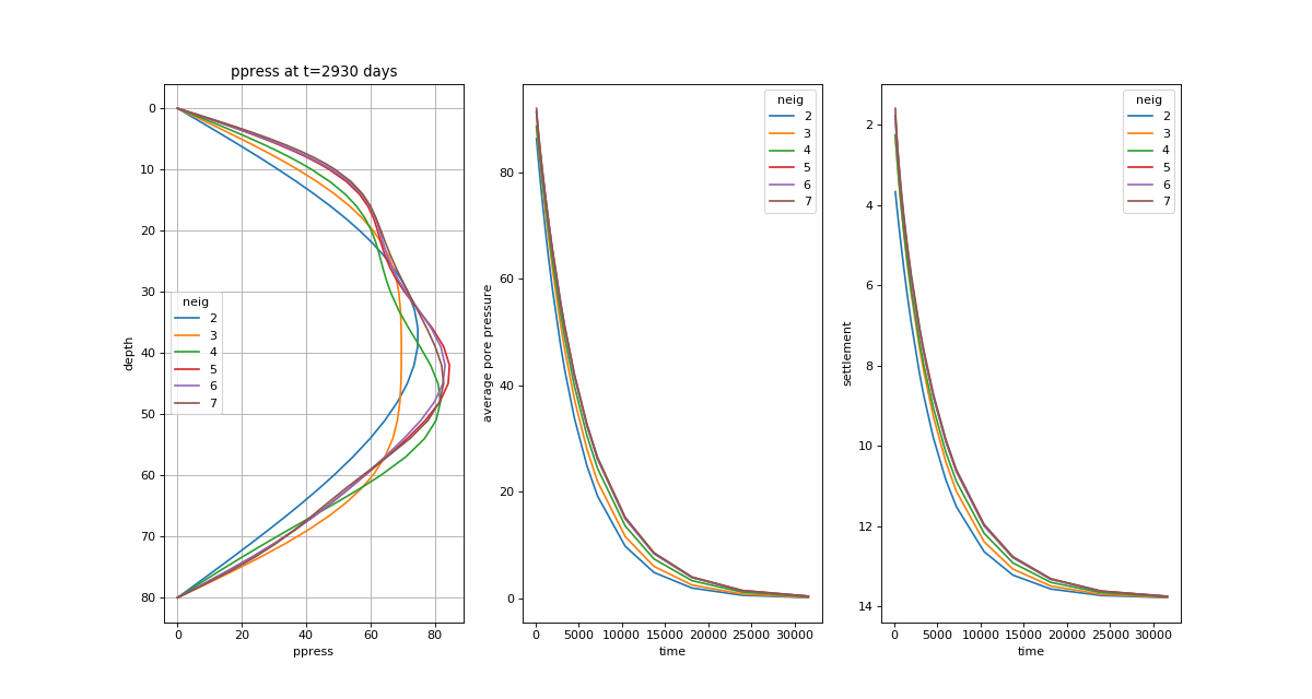
# Examine the effect of number of series terms on pore pressure profiles
# on example_1d_vr_001_schiffmanandstein1970.py

import numpy as np
from geotecha.speccon.speccon1d_vr import Speccon1dVR
import matplotlib.pyplot as plt



fname = "example_1d_vr_001_schiffmanandstein1970.py"
tindex = 11 # time index of pore pressure profile to plot.

with open(fname) as f:
    template = f.read()

fig = plt.figure(figsize=(15,8))
ax1 = fig.add_subplot('131')
ax1.set_xlabel('ppress')
ax1.set_ylabel('depth')
ax1.invert_yaxis()
ax1.grid()

ax2 = fig.add_subplot('132')
ax2.set_xlabel('time')
ax2.set_ylabel('average pore pressure')


ax3 = fig.add_subplot('133')
ax3.set_xlabel('time')
ax3.set_ylabel('settlement')
ax3.invert_yaxis()



for neig in np.arange(2,8,1):
    # Values in an input file can be overridden by appending the new values.
    # More complicated find and replace may be needed if variables depend
    # on each other.
    reader = (template
              + '\n' + 'neig={}'.format(neig)
              + '\n' + 'ppress_z_tval_indexes=[{}]'.format(tindex)
              + '\n' + 'save_data_to_file = False'
              + '\n' + 'save_figures_to_file = False')


    a = Speccon1dVR(reader)
    a.make_all()

    ax1.plot(a.por[:,0], a.ppress_z*a.H, label='{}'.format(neig))
    ax2.plot(a.tvals, a.avp[0], label='{}'.format(neig))
    ax3.plot(a.tvals, a.set[0], label='{}'.format(neig))

ax1.set_title('ppress at t={:g} days'.format(a.tvals[tindex]))
leg1 = ax1.legend(title='neig',loc=6)
leg1.draggable()

leg2 = ax2.legend(title='neig')
leg2.draggable()

leg3 = ax3.legend(title='neig')
leg3.draggable()

plt.show()

(Source code, png, hires.png, pdf)

Multi-line string

Put the following in a .py file and run it with python. A figure with three subplots should appear.

# Example of using a multi-line string to initialize a Speccon1dVR object
# This is the most flexible approach especially for paramteric studies
# and custom plots.
# Only issues are a) no syntax highlighting because text is with a string,
# b) difficult to debug the code within a string.
# Within the string limited calculations are available, outside the string
# in a normal python environment you can do whatever calculations you want
# and place the results in the string.

# Vertical consolidation of four soil layers
# Schiffman, R. L, and J. R Stein. (1970) 'One-Dimensional Consolidation of
# Layered Systems'. Journal of the Soil Mechanics and Foundations
# Division 96, no. 4 (1970): 1499-1504.

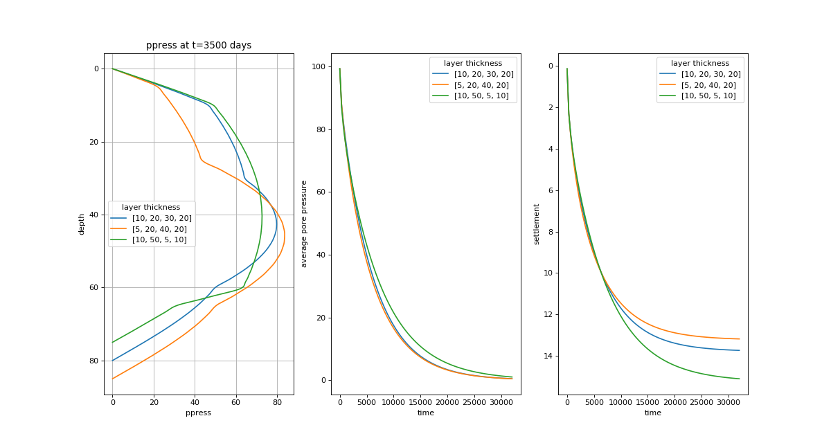
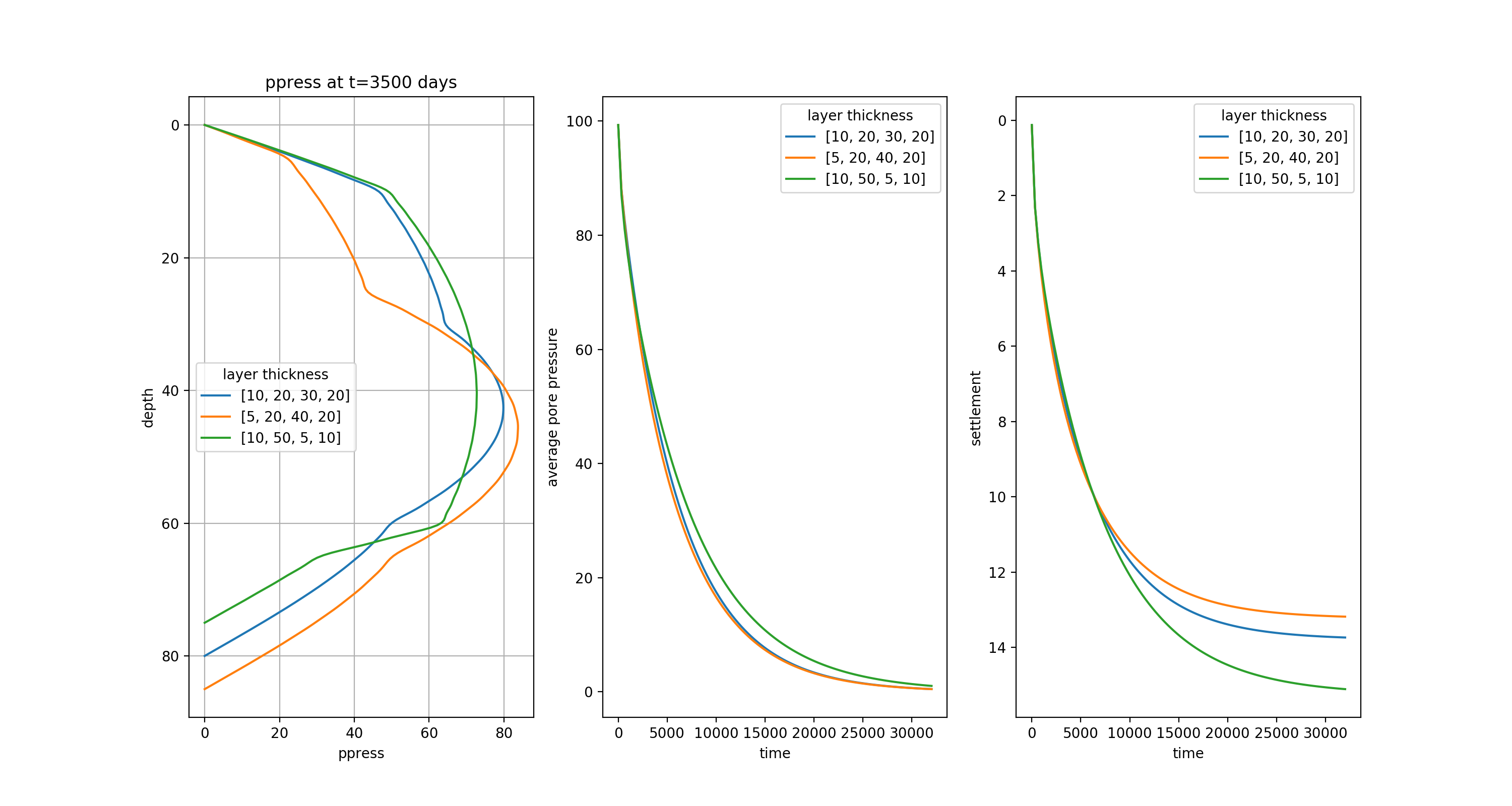
# Examine the effect of different layer thicknesses

from __future__ import division, print_function
import numpy as np
from geotecha.speccon.speccon1d_vr import Speccon1dVR
import matplotlib.pyplot as plt

# changing parameters
h_values = [np.array([10, 20, 30, 20]),
            np.array([5, 20, 40, 20]),
            np.array([10, 50, 5, 10])] # layer ticknesses
tprofile = 3500 # time to calc pore ressure profiles


# the reader string is a template with {} indicating where parameters will be
# inserted.  Use double curly braces {{}} if you need curly braces in your
# string.
reader = """\
# Parameters from Schiffman and Stein 1970
h = np.{h} # article has np.array([10, 20, 30, 20]) # feet
cv = np.array([0.0411, 0.1918, 0.0548, 0.0686]) # square feet per day
mv = np.array([3.07e-3, 1.95e-3, 9.74e-4, 1.95e-3]) # square feet per kip
#kv = np.array([7.89e-6, 2.34e-5, 3.33e-6, 8.35e-6]) # feet per day
kv = cv*mv # assume kv values are actually kv/gamw


# speccon1d_vr parameters
drn = 0
neig = 60

H = np.sum(h)
z2 = np.cumsum(h) / H # Normalized Z at bottom of each layer
z1 = (np.cumsum(h) - h) / H # Normalized Z at top of each layer

mvref = mv[0] # Choosing 1st layer as reference value
kvref = kv[0] # Choosing 1st layer as reference value

dTv = 1 / H**2 * kvref / mvref

mv = PolyLine(z1, z2, mv/mvref, mv/mvref)
kv = PolyLine(z1, z2, kv/kvref, kv/kvref)

surcharge_vs_time = PolyLine([0,0,30000], [0,100,100])
surcharge_vs_depth = PolyLine([0,1], [1,1]) # Load is uniform with depth



ppress_z = np.linspace(0,1,200)

tvals = np.linspace(0.01, 3.2e4, 100)
i = np.searchsorted(tvals,{tprofile})
tvals = np.insert(tvals, i, {tprofile})
ppress_z_tval_indexes=[i]

avg_ppress_z_pairs = [[0,1]]
settlement_z_pairs = [[0,1]]

author = "Dr. Rohan Walker"
"""






fig = plt.figure(figsize=(15,8))
ax1 = fig.add_subplot('131')
ax1.set_xlabel('ppress')
ax1.set_ylabel('depth')
ax1.invert_yaxis()
ax1.grid()

ax2 = fig.add_subplot('132')
ax2.set_xlabel('time')
ax2.set_ylabel('average pore pressure')


ax3 = fig.add_subplot('133')
ax3.set_xlabel('time')
ax3.set_ylabel('settlement')
ax3.invert_yaxis()



for h in h_values:
    a = Speccon1dVR(reader.format(h=repr(h),
                                  tprofile=tprofile))
    a.make_all()
    label='{}'.format(str(list(h)))
    ax1.plot(a.por[:,0], a.ppress_z*a.H, label=label)
    ax2.plot(a.tvals, a.avp[0], label=label)
    ax3.plot(a.tvals, a.set[0], label=label)

leg_title='layer thickness'
ax1.set_title('ppress at t={:g} days'.format(tprofile))
leg1 = ax1.legend(title=leg_title,loc=6)
leg1.draggable()

leg2 = ax2.legend(title=leg_title)
leg2.draggable()

leg3 = ax3.legend(title=leg_title)
leg3.draggable()

plt.show()

(Source code, png, hires.png, pdf)